Introduction
When someone thinks of a texture, they probably think of an image used to 'paint' a model in order to give it a certain appearance. This refers to bitmapped textures, because the texture is made of pixels from an actual bitmap image. These can be very realistic, especially if taken from photographs of actual surfaces. However, one major restriction applies to bitmapped textures: a bitmapped texture has a fixed amount of detail. It cannot be scaled larger without looking softer, it will never yield any more detail than what is already captured in the pixels.
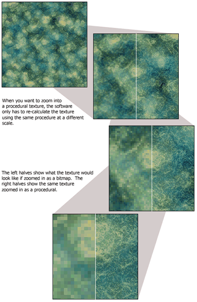
Procedural textures take an entirely different approach. Instead of creating an image by defining a large, unchanging block of pixels, procedurals create the texture from the ground up. This is where the term 'procedural' comes from. The texture is defined only by the procedure needed to create it. You only need to give the computer a (relatively) small formula, instead of a huge block of pixels. With this formula, the computer is able to create the texture at any scale, in any orientation, extending as far as you need.
 Using
these techniques, 3D software is armed and ready to synthesize an infinite
number of textures at your command. Simply tweaking a few parameters can
vary the texture widely. You can think of these textures as space full of
unique shapes and features, extending in all directions, waiting to be explored.
The features in this space are all defined by the interactions between a
set of formulas. These formulas take in a particular coordinate, and they
will report back what sort of feature is at that coordinate. In our case,
these features are colors, and we put those colors on a 3D model.
A procedural function will take a coordinate, and give a color back. A particular function may also have any number of dimensions to it. That is, a 2D procedural, being most like a bitmap image, takes two coordinates, one for X and one for Y, and returns a color. This can be thought of like looking up the color of a pixel in an image. What's the difference? First, n the case of an image, the pixel must be stored explicitly in memory in order to be sampled. As a procedural, the color value doesn't "really" exist until it is sampled, since it is pulled from a formula. Second, again in the case of the image, the space between pixels is undefined. There are only so many pixels in an image, and if you want to see more than that, too bad. In contrast, a procedural texture will let you take a sample anywhere. This is what gives it one of its most remarkable qualities.
It is easier to show some of the results of using procedural textures rather than simply talking about their benefits, so here are four examples of using procedural textures in an actual scene.
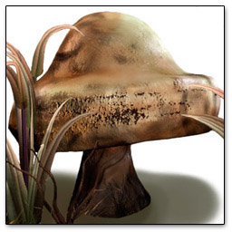
Example 1
This mushroom is entirely textured with procedural functions. It uses a 3D noise function to drive its surface bumpiness. Its color variations are created by a volumetric "billow" function, remapped by a color gradient of various browns and tans. The specular highlight strength is varied by a smooth, low-frequency noise function, in order to give the surface a more natural inconsistent shine. Finally, the contrast of the color function is modified by the slope of the surface, so there is a blotchy pattern along the rim where the slope is extremely vertical.
This texture, which took very little time to design, is very robust and requires no UV mapping at all. It takes relatively little processing power to compute and needs no external image files.
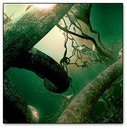 Example 2
The bumpiness on the neurons is created by two voronoi textures blended together at two slightly different sizes, used as a bump map. This is able to give the neuron surfaces a wrinkly, pitted look commonly attributed to photographs in microscopic scale. The same texture is also used to modify the specularity of the texture, so as to limit how shiny the pits will be. This increases their apparent depth. There is a larger 3D noise texture at about five times the scale of the voronoi texture to give a broad, large-scale color variation. If this had been left out, the neurons would have appeared very bland and noisy from a distance (or, to quote Ken Perlin slightly out of context, like salt without food).
It would have been extremely difficult to texture a scene like this with image maps, due to the complex and convoluted surface shapes involved. Where I was able to simply define a few 3D volumetric textures, map their values to colors, and apply them to the entire scene with procedurals, using image textures would have requried me to UV map the neurons and tile textures over their surfaces. Not only would this have been much more tedious, it would have also looked a lot worse without extra work.
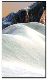 Example 3
Here, procedural textures also allow me to automatically give a surface-feature-based appearance to an object, much like the blotches added to the mushroom when the vertical slope was high.
In this example, the look of wet snow and ice were added to the top of the '"rock" by using the facing direction of the surface. Where the surface faced up towards the sky (Y+), a second procedural texture resembling snow and ice was added to the base procedural texture. The base procedural texture was also slightly darkened to resemble a diffuse shadow cast by the snow where there were breaks in the snow texture. Finally, the dry, powdery snow teture on the ground was created by a noise function scaled up along Z (east-west) to make it appear wind-blown in one direction.
All of these functions are automatic and require very little extra attention of the artist in order to make them work on any surface. In extremely large scenes consisting of many of the same objects (for example, a scene showing miles of rocks in snow), procedural texturing methods are almost essential.
Procedurals need not only apply to shader attributes, but they may be used to sculpt the actual geometry of a surface, as seen in the last example.
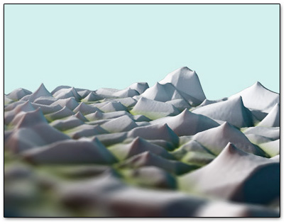 Example 4
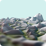
This image of a strange, surreal landscape was created with the output of only one procedural function. The function is commonly referred to as a Worley procedural, named after Stephen Worley, who has done a lot of work on creating cellular texture functions. The Worley procedural is very closely related to Voronoi textures, and is in fact a clever variation of one.
This landscape was originally just a flat plane, but has been displaced by a large-scale Worley texture. The color comes from the same texture, where it has been remapped to a green-to-gray gradient. There are no other textures involved.
Functions
Function Basics
This page may not be of interest to you, and you may safely jump to the next page, "Frequency and Scale"
All procedural textures are functions. You need to tell the texture where on the surface you are coloring in order for them to give back the proper color or value. In other words, you give the function a set of coordinates, and it gives you back a value. Just how many dimensions and how many values depends on the function. A full-color procedural texture will give three values, one each for R, G, and B.
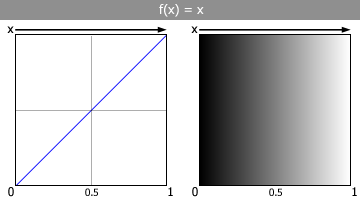
Let's start with a very simple procedural texture. This texture is one-dimensional, and essentially makes a straight (linear) gradient from one side to the other. This texture is defined like this:
f(x) = x
When we give it a coordinate x, it just returns x right back to us.
On the left-hand box, the horizontal direction is the value of x, with the right side being highest (1) and the left side being lowest (0). The gray lines represent halfway marks (0.5). The vertical direction represents f(x), which is the value the function gives back when we give it x. The top is obviously highest, and the bottom is lowest. The right-hand box shows this same function plot as pixel values. Higher values give brighter pixels, where 1.0 is white, and lower values give darker pixels, where 0.0 is black. |
|
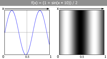
The sine wave is swinging from 0 to 1 so we can see the whole wave. Sine waves are used to make all sorts of nice looking patterns, sometimes alone, and sometimes used as the 'base' for more complex patterns, such as marble veins and wood grain. They are often used with excellent results in many types of plasma or gaseous patterns, and are also well suited for making glows and burst patterns. Although I brought the sine wave's range into 0 to 1 from -1 to 1, I only did that for visual purposes. Sometimes it really is useful to have a sine wave working in this range, but often times it is more useful to keep the sine wave in its natural range. These functions work nicely, and are easy understand, but they are too predictable. Things in nature are irregular. They don't often repeat, at least not in a straight-forward way. The greatest tool we can use in graphics to produce this irregularity is noise. Noise is controlled randomness. There are several types of noise which can add a dash of irregularity to our textures, however, I'm going to focus on a specific (and very popular) type of noise called Perlin Noise, developed by Ken Perlin in the early 1980s. |
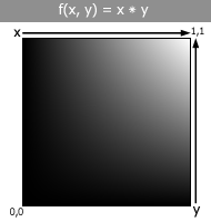
Noise gives us a sort of natural unpredictability to work with. We can use this unpredictability to drive the attributes of more regular functions in order to achieve interesting results. In order to move on, it is necessary to introduce two-dimensional functions. These simply take two parameters, x and y, instead of just x, but still give back one number. In order to further explain this, I'm going to go back to a simple example very similar to the first one I showed you in one dimension: f(x, y) = x * y |
We could take this idea a little further and try using a sine wave on one parameter, but keep the other parameter the way it is. For example, let's try replacing x with sin(x * 10), to get the function f(x, y) = sin(x * 10) * y. |
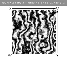
How do we begin to break up these bland, smooth functions with noise? Well, we can start by pushing around the inputs to some of these functions with our noise function. For example, instead of making sin() produce a number directly from the x coordinate, we could push the x coordinate around with a small amount of noise. This is essentially the main approach to building procedural textures: use one function to modify another function until you get the desired result! As I will be demonstrating, many common procedural textures are made this way. Most marble vein textures are made by pushing the x in sin(x) around with a 2D noise function. In this case, the sin(x) function is also usually squeezed into the range of 0 to 1. The entire function looks like this: f(x, y) = (1 + sin( (x + noise(x * 5 , y * 5 ) / 2 ) * 50) ) / 2 This might seem complex at first, but it's easy to understand. Let's look at it in a broken down way.
We multiply x and y in noise(x * 5, y * 5) by 5 in order to make the noise features smaller (by making the coordinates take a stride 5 times larger). We are dividing noise(x * 5 , y * 5 ) by 2 in order to lessen it's effect on x. The less we divide noise(x * 5 , y * 5), the more rough and wild the marble veins will become. We then multiply the result of that part by 50 to increase the frequency of the sine waves. The rest of the function, where we add 1 at the beginning, and divide by 2 at the end, puts our sin() function into the range of 0 to 1. What does this look like? |
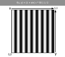
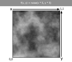 (Left)
The sin() function alone, with no noise to modify
the x parameter.
(Right) The noise() function alone.

Finaly something more interesting! The normally boring 1D sin() function is now being wobbled about its x parameter by a 2D noise() function. We could potentially remap these grayscale values to colors, or add them to an already existing noise texture, to get even better looking results.
|
Big Picture
Frequency and Scale
Procedural textures are all about the details. Detail doesn't just mean the small things, it refers to any part of "the big picture" which can be looked at separately from the rest. A good procedural texture will be made up of details at many different scales; it will have large sweeping details, medium sized details, tiny details, even tinier details, and many in between.
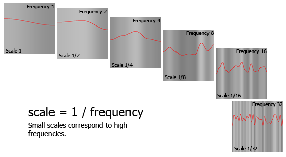 Look
at these scales as frequencies, like the frequencies in an audio wave. The
highest frequencies carry all the information about how the wave moves on
the smallest scales, while the lowest frequencies represent the widest, slowest
variations. Thinking about this, you can see that scale is the inverse of
frequency.
Apply this concept to the earth. The largest scales represent the oceans and continents. These objects have the most obvious shape on a very large scale. As you get closer, however, their large-scale shape becomes unnoticable, and you see the smaller scales fade into sight, forming mountain ranges, coastlines, forests, and deserts. You move in closer, and begin to notice even finer details, including groups of individual trees, large buildings, and rivers. All of these shapes and features can be considered on independent scales, but are all part of the same earth.
 The
idea that "the big picture" is formed by several levels of combined
detail was probably in the minds of many artists and philosophers over the
millennia, however it was first put into practical use in the early 1800s
by Joseph Fourier. Fourier discovered the concepts of Fourier Analysis, which
essentially states that any function can be approximated by the sum of sine
and cosine waves over a range of different frequencies and amplitudes (whew).
This idea was found to apply to just about everything, including audio and
imagery.
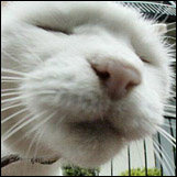 Let's
take the face of this cat, for example.
The area around its mouth is noticably darker than the rest of its face. The light intensity there drops smoothly over a width of about 45 pixels, and then goes back up.
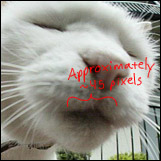 Look
at this as the result of a function, with a 45 pixel scale, lowering the
brightness at this spot.
What happens if we separate this image into various scales (see the images to the left), putting it back together, except leaving out the scales responsible for 32-pixel and 64-pixel wide details?
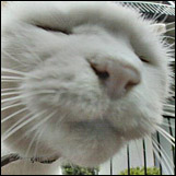 The
mouth area is no longer darkened, because there is no longer any variation
at the necessary scale. The bright spots on the fur have also become dull,
since their detail fell within roughly the same scale. Obviously, it is very
important to make sure your texture contains variation at all scales,
or you will lose the richness afforded by subtle variations in color and
brightness.
Some painters tend to work in a very similar manner. To begin their work, they will paint out large vague blobs of color. Slowly they will make repeated passes over the blobs, each time adding another level of definition, gradually building up shape and detail, until they are down to filling in the very finest details they are able to paint. When you're doing procedural textures, since one detail level doesn't disrupt the other, it is generally okay to work in either direction, that is, you may start small and go big, or start big and go small.
Here are some simple, boring functions which, when repeatedly combined with smaller and smaller versions of themselves, create very interesting patterns. The table below shows you the basic source pattern (left), and combinations of that pattern with smaller versions of itself using various combination methods.
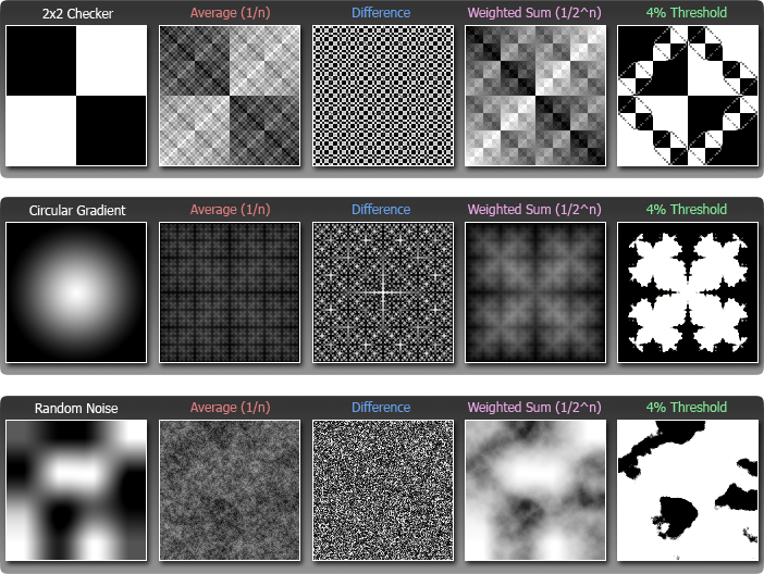
Average (1/n) - This is simply the average of all of the scales being used, 'n' is the total number of scales. So if there are 6 scales, each scale contributes about 16% (1/6th) of the final value.
Difference - This uses the difference between the color values of each scale as the final texture color.
Weighted Sum (1/2^n) - The weighted sum is very similar to the average, except the larger scales have more weight. As 'n' increases, the contribution of that scale is lessened. The smallest scales (highest value of n) have the least effect. This method is the most common and typically the most visually pleasing.
4% Threshold - This is a version of the Weighted Sum where anything below 48% gray is turned black, and anything above 52% gray is turned white.
The process of combining several copies of the same thing at different scales is also sometimes called 'Fractal Synthesis'. This is where fractals get their name, they are created by iterating over and over through the same function on different scales, which gives them their interesting self-similarity.
Types Of Textures
Voronoi
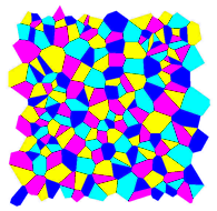
A Voronoi diagram is a diagram that contains a set of points and a set of edges. The edges partition these points in such a way that, if you were to pick a random location in the diagram, and look at which set of edges you're inside, the location you chose is closest to the point inside those edges than any other point in the diagram. The edges in a voronoi diagram lie in the places where a location is equidistant to two or more points.
Think of it as if you had a set of randomly colored, randomly located points. Suddenly, these points start growing into circles, and expand until they meet. Where these circles meet, they stop growing, but they keep expanding where they haven't touched anything, until all space is filled up. As a result, you'll get a bunch of randomly colored fragments of geometric shapes. These shapes define the voronoi regions for their points; in other words, every location inside a given shape is closest to that shape's "birth point" than any other point.
In actuality, Voronoi regions are computed in an entirely different manner. They can be computed in several ways, in fact. The easiest way is simply to pick a location, find out which random point you're closest to, and then say "hey, alright, this location is inside this point's Voronoi region!"
The patterns defined by Voronoi regions show up everywhere in nature. In biology, cells pack together in a very similar manner. When you have a bunch of soap suds, the intersections where bubbles meet and merge together form Voronoi regions. On a frosty pane of glass, frozen water vapor expands into Voronoi-like shapes.
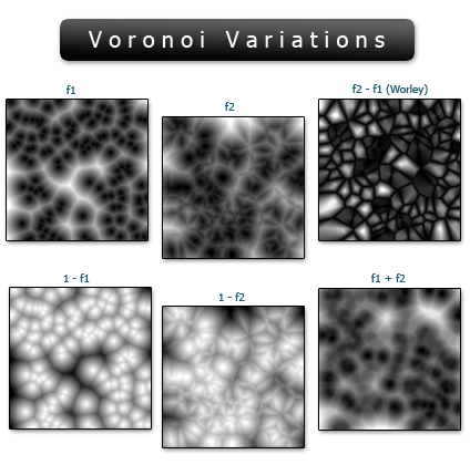
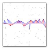
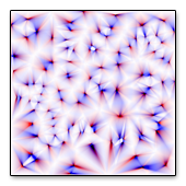
When computing a Voronoi texture, you pick a pixel, and find the point closest to that pixel. The pixel's color is determined by the distance to that point. You can make variations of the texture by instead using the second closest point, or third, etc. There is a naming convention for variables used to represent the distance from a pixel to a point. Typically, "fn" is used, where n is the nth closest point to the pixel being sampled. For example, f1 would be the distance from the pixel to the 1st closest point, f2 would be the distance to the 2nd closest point, and so on.
Animated Examples (Java, Pop-Up)
|
This example shows f1 (red) and f2 (blue) lines stretching from a row of pixels to their 1st and 2nd closest points. These lines represent the distance from each closest point to each pixel in the row, which is controlled by your mouse cursor. The color of the pixels in that row, if they had been drawn, would be brighter as the lines got longer. |
Nearly identical to Example 1, except the distance lines accumulate and blend together as they are drawn, so you are able to see them leading to every region in the image at once. |
Common Terms
| f1, f2, ...., fx | Used to denote '1st closest', '2nd closest', ..., 'x closest' point distance. |
| Manhattan Distance |  This
method uses orthogonal (90 degree) lines instead of straight lines to
calculate the distance between samples and points, named so because the
method resembles city streets. This
method uses orthogonal (90 degree) lines instead of straight lines to
calculate the distance between samples and points, named so because the
method resembles city streets. |
| Distance Squared | A distance modification used to effectively smooth out pointy, cone-like features in the texture. |
Noisy Finish
Noise
 Noise
is the holy grail of procedural textures. It is one of the first functions
used to destroy the plastic appearance of computer graphics with the power
of unpredictability. The computation of noise is also a deep subject; true
noise should be completely random, but generating random numbers on the computer,
which is a machine of the most strict order, is a very complex task.
Noise itself comes in many forms, but all have the same goal: irregularity. It is used in most textures as a function for introducing irregular patterns and distributions. The most basic form of noise is usually caled "Salt and Pepper" noise, which is characterized by simply choosing a 0 or a 1 randomly for every single sample.
The most important feature of noise in computer graphics is pseudo-randomness. This means if we give the noise function a certain input number, it will always return the same random result for that number. In this sense, it is not truly random, but that's a good thing. If we're sampling the random value for a certain pixel, it won't change every time we sample it.
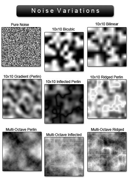
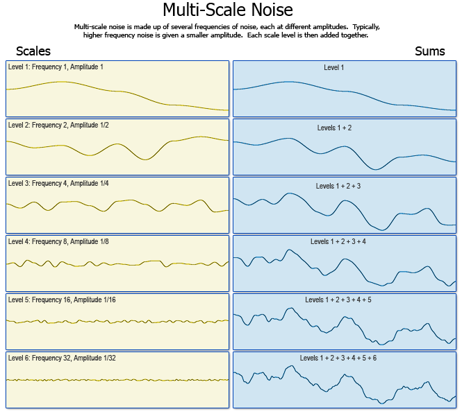
Multi-scale noise functions are typically the most useful. They're created by adding together several basis functions at different scales and amplitudes.

Basis Function for standard Perlin Noise

Basis Function for Ridged Perlin Noise (1 - abs(noise))
Below is an example of how consecutive scales are added together to create a complex multi-scale noise function. The left column shows each scale in succession, while the right column shows the noise function in various levels of complexity.
Common Terms
| Frequency | The base frequency of the texture. Higher frequencies result in smaller features. |
| Inflection | This refers to taking the absolute value of the noise function, resulting in sharp discontinuities where the function meets 0. This gives the noise a bubbly look. Subtracting the absolute value from 1 instead flips the values around, giving the noise a ridged look. |
| Lacunarity | In multi-scale noise, lacunarity is the spacing between consecutive scales. Typical noise uses a lacunarity of 2.0, which means the noise will be made up of scales at 1, 1/2, 1/4, 1/8, 1/16, 1/32, 1/64 ... 1/2^n. Reducing the lacunarity to 1.0 effectively makes it a single-scale noise function, since 1/1^n is always going to be 1, no matter what n is. |
| Persistence | In multi-scale noise, persistence refers to the amount of contribution smaller scales make to the overall texture. A higher persistence will result in a noisier, more complicated looking texture, where the fine details are strong and drastic. This is also sometimes referred to as the fractal dimension. |
| Octave | An octave refers to the level of scale of a function. For example, the first octave in a function represents a scale of 1. The second octave represents a scale of one-half (or, a frequency of 2). Each successive octave is half the scale of the previous. In music, an octave refers to a musical interval of eight tones, which is a very closely related concept. |

 Tutorials
 This
means where the x coordinate
in the image is higher, the texture is lighter. The y coordinate
is not used, since this is a 1D texture, so it has no effect. This
texture function looks exactly the same on the top as it does on the
bottom.
 This
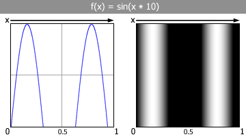
one is a tad more interesting. It uses a sine wave driven by x,
but x is multiplied
by ten in order to bump the frequency up. Notice it doesn't look exactly
like a sine wave, but more like two humps. This is because the rest of
the sine wave is hidden below zero, since sine waves go from -1 to +1.
Let's try and fix this. First we want to get the sine wave to be above
zero. So, since it dips below zero by -1,
let's add 1 to it. This will make the sine
wave now swing from 0 to 2 instead
of -1 to 1.
Next, to get it down in the range of 0 to 1,
we divide it by 2.
  And
it worked just fine!
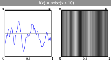 I'm
not going to explain how perlin noise works right now, that is best
left to another document, or you could just read the
  In
this example, you can see the brightest point is where both x and y are
equal to 1. This is because the formula
is x * y,
and 1 * 1 = 1. Remember 1 is
white and 0 is black. At the upper left
and lower right corners, one parameter is 1 but
the other is 0, and anything times 0 is 0.
So we have a texture that gradually gets brighter as x and y approach
1 together.
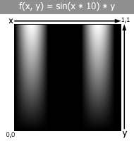 It
looks almost exactly like the one-dimensional f(x)
= sin(x * 10) example I showed earlier,
however it fades out as y drops,
thanks to the "* y" addition.
This makes the texture officially two-dimensional.
